Compensating for hardware limitations#

Make no mistake: any engineer can tell you that the BrachioGraph is no way to build a plotter. Hobby servo motors are under-powered, imprecise and not designed for this kind of job. Ice cream sticks lack rigidity. The pen-lifting mechanism tends to move the pen sideways. And so on.

That is partly what makes it fun, that it does things its parts are not ideally suited to, and does them well enough to make the results interesting and worthwhile in their own right.

To get the best results involves understanding the limitations of the hardware, and finding ways to compensate for them.

About the servo motors#

Each servo motor is different, so the BrachioGraph can be calibrated exactly for your servos. To get you started however, it makes some assumptions about the servos.

For SG90 motors or similar:

they have almost 180˚ of rotation, though they are specified for 120˚ and that’s the better value to assume
they operate on pulse-widths from about 500µs to about 2600µs, though the official values are 1000µs to 2000µs and those are better values to use
the centre of their travel is around 1500µs
one degree of travel corresponds a difference of about 10µs

This is what the default angles_to_pw_1 and angles_to_pw_2 methods assume when the BrachioGraph is initialised.

This is sufficient to get started, but since the values above are nominal values only, they won’t provide the best results. In addition, the correspondence between pulse-widths and angles is not actually linear, and worse, mechanical hysteresis in the system means that the quality of your drawings will be much lower than it ought to be.

Non-linearity#

By default, the BrachioGraph assumes a linear response from the motors. This basic form of this naive formula is for the pulse-width required for a particular angle is:

pw = 1500 + angle x 10

(1500µs is the nominal centre of a servo’s sweep, and a change of 10µs generally seems to correspond to 1˚ of movement.)

See the naive_angles_to_pulse_widths methods for how this formula is implemented.

However, servo motors are far from being perfectly linear. A linear relationship between pulse-widths and resulting angles would be a straight line. In practice, they can look rather like this:

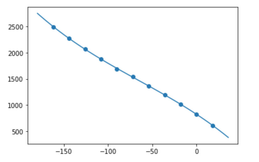
If we know the characteristics of the non-linearity, we can compensate for it. By recording a series of actual pulse-width values and their corresponding angles, we can use Numpy’s polyfit module to obtain a function for this non-linear relationship.

Hysteresis#

The BrachioGraph is susceptible to hysteresis, a tendency of the system to maintain its state. In this case, it means that if the device receives a command to move to a certain point, where it actually arrives can depend on the direction it was coming from.

The motors#

The motors themselves, even more accurate and expensive ones with metal gears and high torque, exhibit hysteresis, even when under no load. For example, say that at 1500µs your motor is at 0˚. You may find that changing the pulse-width from 1500µs to 1510µs moves the arm anti-clockwise by 1˚, but setting it back to 1500µs does nothing, and the motor does not move back to 0˚ until the pulse-width is set to 1490µs.

In other words, the position of the motor at 1500µs is dependent upon the its previous state; in this example it will be 0˚ when moving anti-clockwise and -1˚ when moving clockwise.

The mechanical system#

In addition, the mechanical system - the arms, the joints and the way the pen is held - adds more hysteresis. As the motors move, some of that movement will be taken up by flexing and mechanical free-play in the system, so that the actual relationship between pen position and pulse-width can suffer from a dead-band of more than 15µs when changing directions.

The result of this hysteresis is imprecision that depends on direction. Drawing a grid with the lines first in one direction and then another will make this obvious:

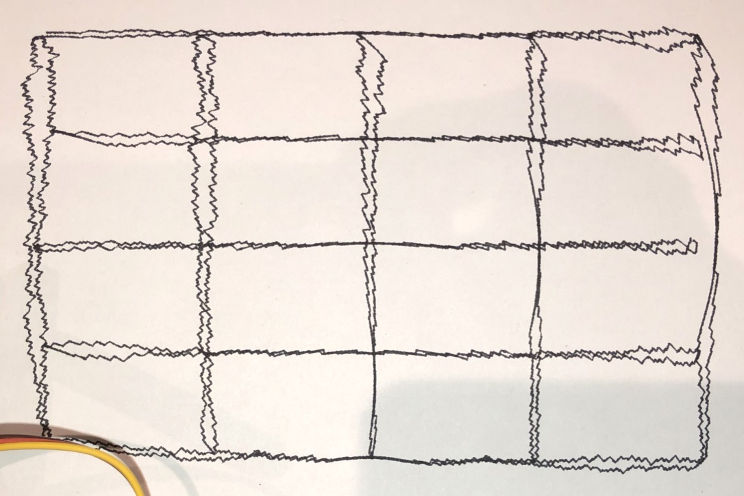
Compensation for hysteresis#

The BrachioGraph can compensate for hysteresis by anticipating it. In the example above, adding or subtracting a constant to the pulse-width value when it is increasing or decreasing will help eliminate the dead-band:

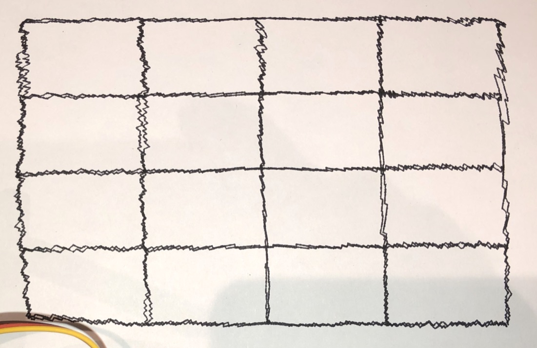
The correction values are supplied as hysteresis_correction_1 and hysteresis_correction_2 parameters to the BrachioGraph instance. See Counteract hysteresis for how to determine these values.

If you’re using more sophisticated calibration using servo_1_angle_pws_bidi and servo_2_angle_pws_bidi, the hysteresis values will be calculated for you.