5. Start plotting

5.1. Move the arms

The set_pulse_widths() method is a manual way of setting the pulse-widths that determine the position of a servo. Try this:

bg.set_pulse_widths(1500, 1500)

Nothing should happen, because those are already the pulse-widths it’s applying. But try incrementing the first servo pulse-width by 100 (microseconds) - make sure you get the numbers right, because a wrong value can send the arms flying:

bg.set_pulse_widths(1400, 1500)

This should move the inner arm a few degrees clockwise.

The first value controls the pulse-width of the shoulder servo, and the second the pulse-width of the elbow servo. Try some different values for the two servos, changing them by no more than 100 at a time, until the arms seem to be perpendicular to each other and the drawing area.

On a scrap of paper, note down those two values; we’ll use them in the next step.

Servo	pulse width at parked angle
Shoulder (parked at -90˚)
Elbow (parked at 90˚)

5.2. Initialise a custom BrachioGraph

By default, a BrachioGraph is initialised with values of 1500 for both servos (for most servos, 1500 µs places them at the centre of their movement). However you probably found that slightly different values are needed to line up the arms at the correct angles. Let’s say the two values you noted in the previous step were:

• 1570 for the shoulder motor

• 1450 for the elbow motor.

In that case, re-initialise the BrachioGraph using the values you discovered:

bg=BrachioGraph(servo_1_parked_pw=1570, servo_2_parked_pw=1450)

5.3. Start drawing

Now you should be able to draw a box:

bg.box(bounds=[-2, 7, 2, 11])

This means: draw a rectangle defined by the co-ordinates -2, 7 at the bottom-left corner and 2, 11 at the top-right corner. Everything is always relative to the shoulder motor’s spindle at 0,0):

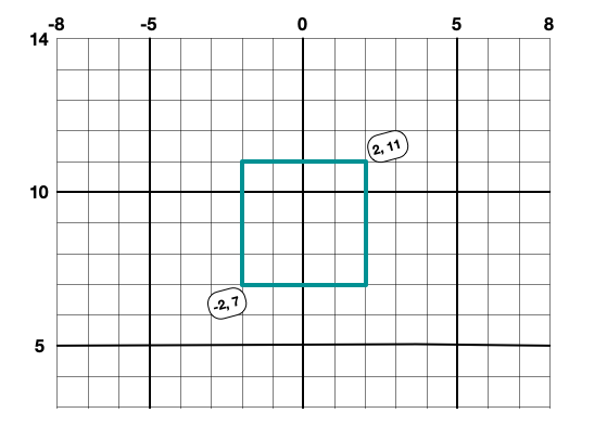
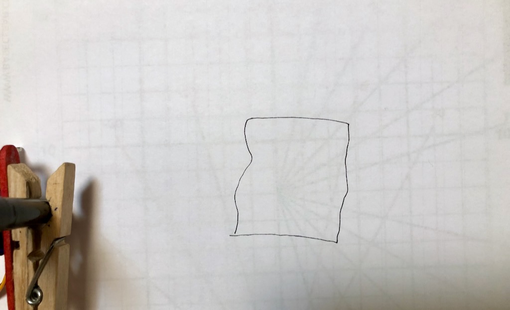
The BrachioGraph will draw your square. It will be a wobbly, imperfect square, but it should be a recognisable square, about 4cm wide and tall:

Try increasing the dimensions of the box progressively, for example:

bg.box(bounds=[-3, 6, 3, 12])

If you’re lucky, you should be able to draw a box that is the full size of the default drawing area. The status() command you used above shows that:

bottom left: (-8, 4) top right: (6, 13)

To draw a box around this area, use the box() command without any parameters:

bg.box()

5.4. Try some test patterns

And now draw a test pattern:

bg.test_pattern()

What happens if you draw the test pattern in reverse?

bg.test_pattern(reverse=True)

You’ll find that the patterns line up very imperfectly. This is because of slack and friction in the system.

In the next section we’ll try to mitigate this, and generally improve the accuracy and precision of the plotter. In the meantime, let’s draw a test image.

5.5. Draw a picture

In the images directory, you’ll find a file called demo.json. This contains the lines and the points along them, represented as co-ordinates in JSON format, and is what the plotter uses to draw

Plot the file:

bg.plot_file("images/demo.json")